raw pvalue distribution

[nservant]

Hi,
I have some results I cannot really explain when looking at the raw pvalue distribution.
Here is my framework from the csaw book ;

param <- readParam(restrict=paste0("chr", 1:22), minq=20)
win.data <- windowCounts(bams, width=2000, spacing=1000, ext=125, param=param)
bins <- windowCounts(bams, bin=TRUE, width=10000, param=param)

## Local filtering
neighbor <- suppressWarnings(resize(rowRanges(win.data), width=5000, fix="center"))
wider <- regionCounts(bams, regions=neighbor, ext=frag.len, param=param)
filter.stat <- filterWindowsLocal(win.data, wider)
hist(filter.stat$filter, main="", breaks=50, 
     xlab="Background abundance (log2-CPM)")
abline(v=log2(2), col="red")
keep <- filter.stat$filter > log2(2)
summary(keep)
filtered.data <- win.data[keep,]

## Normalize on bg
filtered.data <- normFactors(bins, se.out=filtered.data)    

## Differential analysis
y <- asDGEList(filtered.data)
design <- model.matrix(~ 0 + splan.sub$GROUP)
colnames(design) <- c("EGF", "untreated")
y <- estimateDisp(y, design)
fit <- glmQLFit(y, design, robust=TRUE)
contrast <- makeContrasts(EGF-untreated, levels=design)
res.csaw <- glmQLFTest(fit, contrast=contrast[,1])
hist(res.csaw$table$PValue)

And here is my raw pvalues distribution :

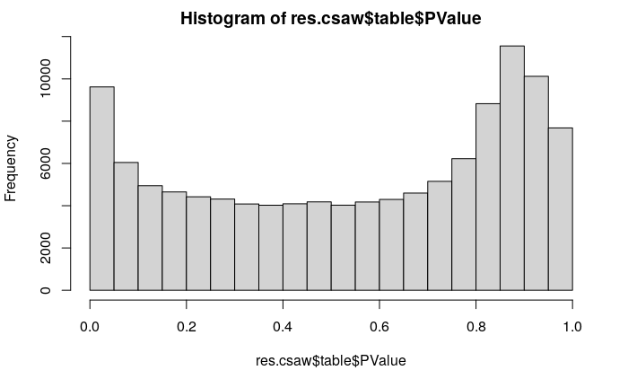
As I do see this peak for extreme pvalues, I decided to be more stringent on the filtering. Usually, from my experience on RNA-seq data, it should help solving this issue.

However, I do have exactly the opposite effect !

keep <- filter.stat$filter > log2(5)
summary(keep)
filtered.data <- win.data[keep,]

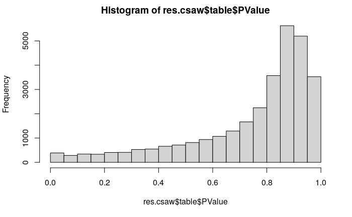
I was wondering how we could explain this behaviour ?
I have the same effect using global/local filtering.
Many thanks

[LTLA]

Enrichment of large p-values is pretty common if you have big IP efficiency differences between replicates. These are emphasized when you use background-based normalization. It's not great but there might not be much that can be done if you need to use background-based normalization, e.g., because of global changes in binding between conditions.

Hard to say what the peak of low p-values are. The background-based normalization should have removed most DB at low abundances, by definition. Perhaps looking at the tracks or genomic context might provide some insight. For example, I remember that microsatellites and other repeat regions were major causes of spurious DE.